How to Use the VLOOKUP Function in Excel Tutorial (20 Quick Guide Cheat Sheets)
Why do Employers look for VLOOKUP skills in their job ads? And why do so many small, medium and large businesses use the VLOOKUP formula in their excel files?

Because not all data are in the same databases or systems. Often data is collected from different systems and is not yet connected in a way so that people can make the right decisions based on these different data sets. VLOOKUP helps to relate data in one table to another table.
For example a business might have a system where customers place orders and another system where customers pay for their orders once received. To compare what these customers finally paid versus the amount of the order billed VLOOKUP can help and save a lot of time by comparing the imported data in two seperated sheets in Excel.
Instead of wasting a lot of your precious time manually comparing data in excel tables and even risking to get it wrong let me show you visually step by step in this tutorial how to use the VLOOKUP function in excel.
Step 1: Where to find the VLOOKUP Formula in Excel?
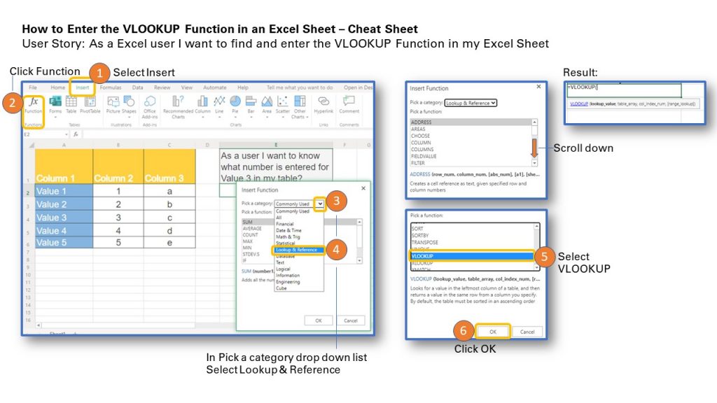
For the first examples I use office 365.
Step 2: How does the VLOOKUP formula work?
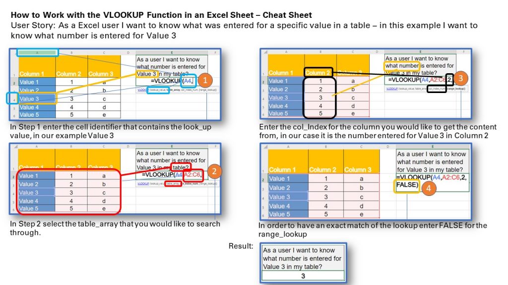
If you want to copy & paste the VLOOKUP formula (Exact Match) example:
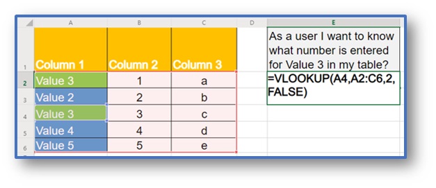
=VLOOKUP(A4,A2:C6,2,FALSE)
Practice Question: What letter was entered for Value 5 in the excel table?
Solution:
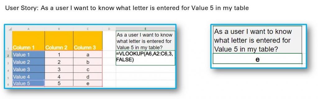
=VLOOKUP(A6,A2:C6,3,FALSE)
Why is this excel function called VLOOLKUP?
Vertical tables always have the data listed below a column.
What is one of the most used vertical tables in your live?
…. probably a calendar.

The V is for vertical, but what is a lookup table? It is a prepopulated array of data which helps to reduce the process time of a computer. It avoids to carry out a data base query each time to compare a value. Before the computer lookup tables help to reduce the effort of calculating values. The most famous example is the logarithmic tables:

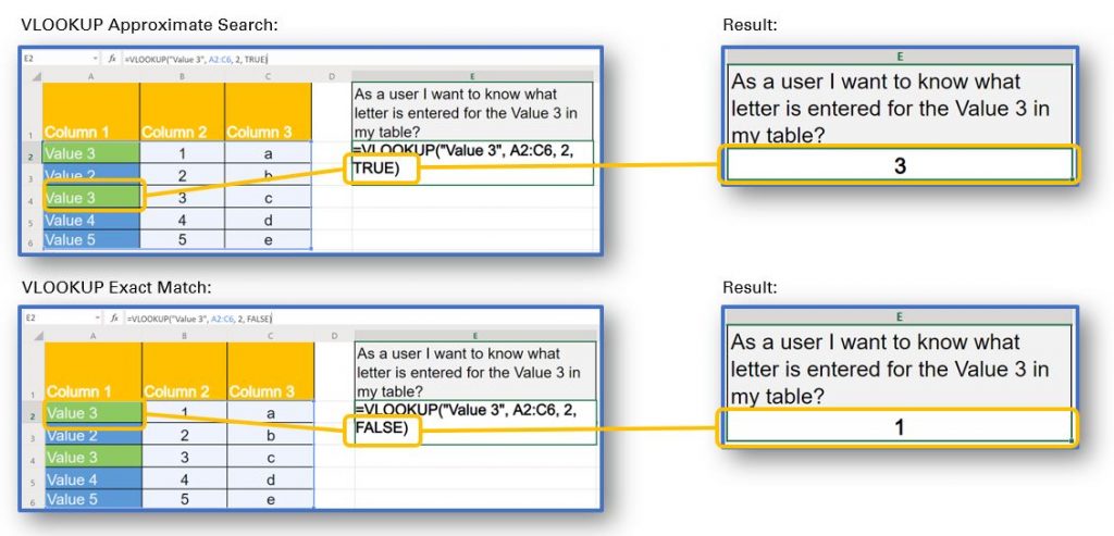
To demonstrate how VLOOKUP is looking vertically through the table I take the VLOOK Cheat Sheet example from the introduction. I add now one twist. Instead of just heaving Value 3 only once in the table it now appears 2 times. I have highlighted it in green color.
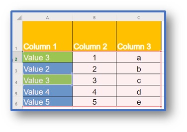
In the introduction of the VLOOKUP function I have used the question: “As a user I want to know what number is entered for Value 3 in my table?” And VLOOKUP returnd the number 3.
What will the answer be this time?
The answer is 1 because VLOOKUP is looking vertically from top to bottom through Column 1.
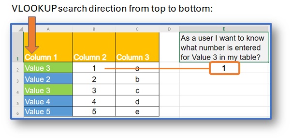
It is always the first match
that VLOOKUP will catch!
“Look to the right side of table” – freely adapted from Monthy Python (“Always look at the bright side of vlookup”)
Let’s put the theory to test – and see if VLOOKUP can look to the left side: As a user I want to know what Value is entered for letter d in my table?
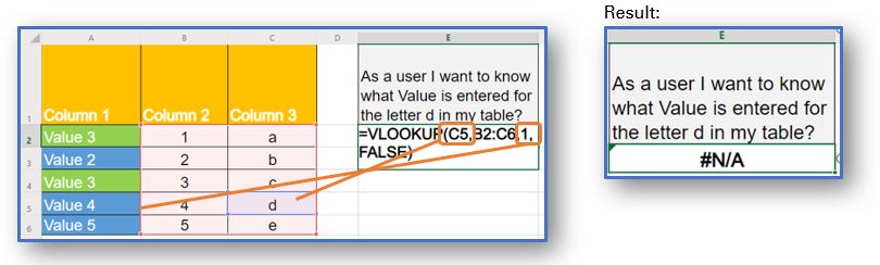
VLOOKUP shows a not found error: #N/A. So the conclusion below:
If you wake up at night- remember:
VLOOKUP only looks to the right
and never to the left side!
VLOOKUP is a LEFTIST
Don’t believe me? – I will show you.
Let’s ask VLOOKUP: As a user of excel I want to see what letter was entered for the number 2 in my table?
Shouldn’t it work because we have just learned that VLOOK always looks to the right side of the table.
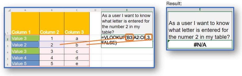
As expected VLOOKUP returns a not found error message: #N/A.
How to fix it?
Remember VLOOKUP is a Leftist. VLOOKUP will always search through the fist column in the defined table_array for the search. The current search is in Column 2 (B) while the table_array is from Column 1 (A) to Column 3 (C). The way to fix it is to change table_array to start in Column 2 in Cell B2 instead of A2. But this is not all! Since the table_array has now only two columns also the col_Index_num to retrieve the value from needs to change. Instead of col_Index_num 3 col_Index_num 2 needs to entered.
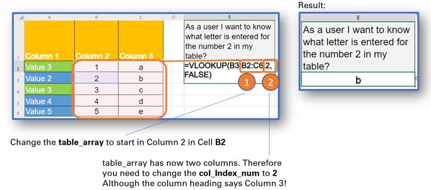
=VLOOKUP(B3,B2:C6,2,FALSE)
VLOOKUP search will be okay
in the first left column of the table_array
If you want to copy & paste the VLOOKUP formula named range example:
=VLOOKUP(E2,Score,2,TRUE)
In Search for a Number
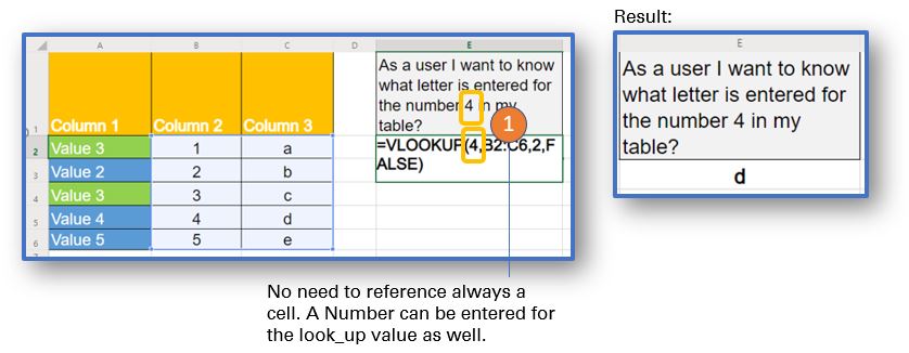
No need to always reference a cell for the look_up value in VLOOKUP. A number to lookup can be entered as well directly in the function.
See the example below: Looking for the number 4 will bring the correct result of the letter d.
If you want to copy & paste the VLOOKUP formula number example:
=VLOOKUP(4,B2:C6,2,FALSE)
In Search for Words
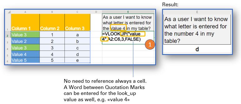
The same applies for words. No need to always reference a cell for the look_up value in VLOOKUP. A test to lookup can be entered as well directly in the function.
There is one difference to search for a number so, you need to entered the word between Quotation Marks.
See the example below: Looking for the “value 4” will bring the correct result of the letter d.
If you want to copy & paste the VLOOKUP formula text example:
=VLOOKUP(“value 4”,A2:C6,3,FALSE)
Did you notice something?
Take it as a positive
VLOOKUP is not case-sensitive
VLOOKUP has a wildcard – The Exact Match versus the Approximate Match
The first to serve is Exact Match.
In the example below Exact Match is asked to look for the number 10 and show the corresponding letter.
It will not surprise you to see the following result:
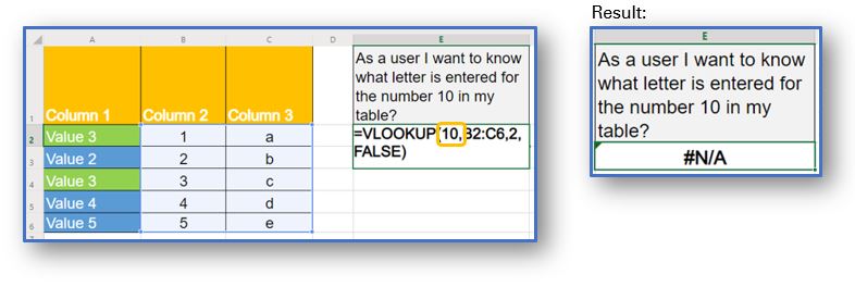
Give me the letter for 10 and VLOOKUP returns #N/A (not found) message.
What needs to change in order to have a hit and not a miss?
The Approximate Match comes to rescue as shown below.
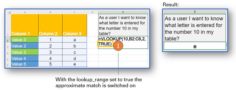
If you want to copy & paste the VLOOKUP formula (Approximate Match) example:
=VLOOKUP(10,A2:C6,2,TRUE)
In the VLOOKUP function the lookup_range needs to be set to TRUE to switch on the approximate match.
The closest match VLOOKUP found for 10 is 5. Therefore VLOOKUP returned the letter e.
How the Approximate Match helps to avoid many If functions?
Let’s assume the following business scenarios: As an HR Employee you have recieved all the performance ratings of the employees you are repsonsible for or as Marketer you have run a servey and now collected all the total scores.
The rating scale used startet at 1 lowest went to 5 highest for all of the ratings. In the HR example employees were rated each several times on different goals and competences and in the case of the marketer the participants answered several questions about a specific offering. So the total score received in these examples will most of the time not be a straigt number.
Example HR | Performance |
| Example Marketing | Rating |
Employee | Score | Participants | Score | |
1 | 4.2 | 1 | 4.3 | |
2 | 4.8 | 2 | 4.5 | |
3 | 3.3 | 3 | 2.8 | |
…. | …. |
Based on the different score the wish is to put them into one of the 5 categories.
From score 1 to 1.9 employees are put in the category a, for 2 to 2.9 in b and so on. The same would apply to the marketing example.
In HR the category a-e would decided on the next pay increase the employee will get. In Marketing the categories could define for example what type of people (segment) would value the product most.
Solving the problem first with the If Function:
If you want to copy & paste the nested IF function example:
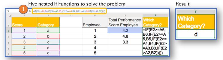
=IF(E2>=A6,B6,IF(E2>=A5,B5,IF(E2>=A4,B4,IF(E2>=A3,B3,IF(E2>A2,B2)))))
In this example five nested If Functions are required to select the corresponding category. Now imagine doing this for 10 Categories.
Luckily VLOOKUP can do the same and it will be much easier to enter then 5 nested If functions. Just see with your own eyes below:
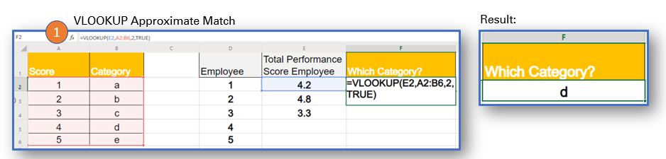
If you want to copy & paste the VLOOKUP formula (Approximate Match) example:
=VLOOKUP(E2,A2:B6,2,TRUE)
Instead of writing 5 If Functions: =IF(E2>=A6,B6,IF(E2>=A5,B5,IF(E2>=A4,B4,IF(E2>=A3,B3,IF(E2>A2,B2)))))just using the VLOOKUP Approximate Match: =VLOOKUP(E2,A2:B6,2,TRUE) will deliver the same result.
Before using If this then that
use VLOOKUP Approximate Match instead
Calculating the sales commission is another example where the VLOOKUP Forumula with the Approximate Match is useful.
Based on the amount of sales in a month, quarter or year the percentage of the sales commission is defined based on a range, e.g. Sales below 10 000 USD will recieve a 1% commission, Sales below 50 000 USD will recieve 2%, and so on.
How to avoid problems when copying the VLOOKUP Function?
Let’s follow through on our last example of the VLOOKUP Approximate Match formula.
First let’s add data for employee 4 and 5 and second let’s copy the formula =VLOOKUP(E2,A2:B6,2,TRUE) to the next 4 lines in our table.
And this is the result:
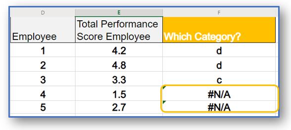
While all went well till line three, line 4 and line 5 show a not found error #N/A.
What went wrong?
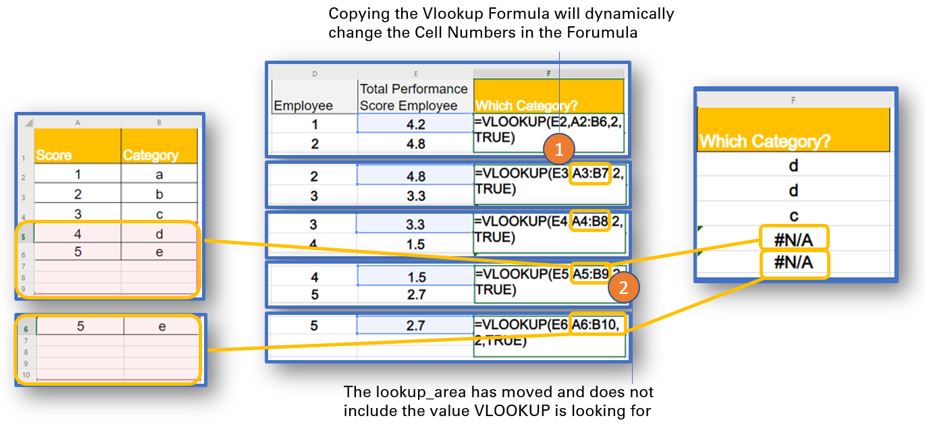
When copying the VLOOKUP formula as it is written now =VLOOKUP(E2,A2:B6,2,TRUE) to the next line will cause the cells to dynamically change. This impacts also the lookup area. The area moves from A2:C5 step by step to A6:B10. Finally this will cause the error for employee 4 as the performance score 1.5 is not anymore found in the lookup area. VLOOKUP returns a not found error #N/A.
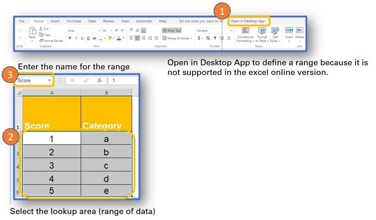
How to solve this issue?
see below
How to name a range in Excel?
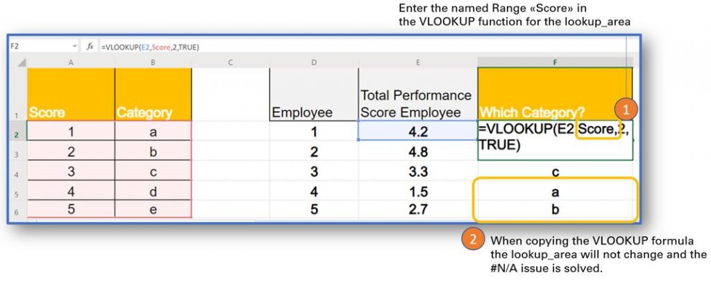
As shown below copying the VLOOKUP formula with a named range will not change the lookup_area. Therefore the correct category will now show for Employee 4 and Employee 5.
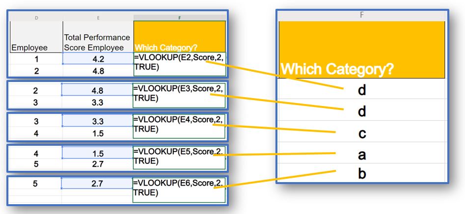
If you want to copy & paste the VLOOKUP formula named range example:
=VLOOKUP(E2,Score,2,TRUE)
IF VLOOKUP behaves strange
better use a named range
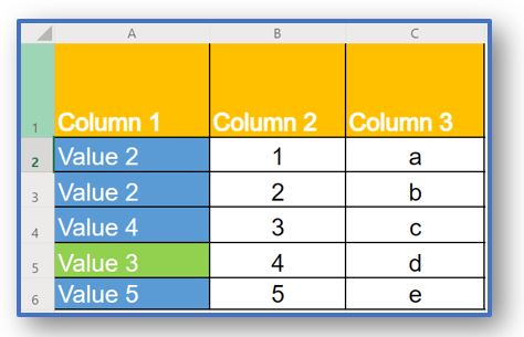
VLOOKUP Approximate Match vs the VLOOKUP Exact Match
VLOOKUP Approximate Match will deliver the result 3 while the VLOOKUP Exact Match will show 1 as the result. Isn’t this strange? Why did VLOOKUP Approximate Match overlook the first Value 3 (Cell A2) and instead went to the Value 3 in the Cell A4?
Because VLOOKUP Approximate Match will use a different search method than VLOOKUP Exact Match.
VLKOOKUP Exact Match will start at the top (in this example in cell A2) and then decend row by row until the correct Value is found, while VLOOKUP Approximate Match uses the binary search method.
To demonstrate it, see below example:
What number will the VLOOKUP Exact Match deliver for the lookup value: “Value 3”?
VLOOKUP Exact Match will start in cell A2 and check Value 2 equals Value 3 which is not the case and move to the next cell A3 and do the same comparision again. In Cell A5 it will find the match and return the result 4.
But what result will the VLOOKUP Approximate Match show?
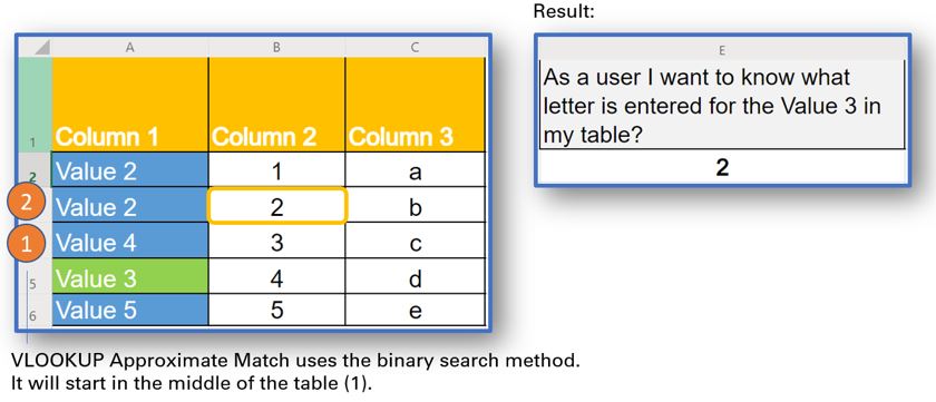
In the binary search method the search will always start in the middle of the table, e.g. in Cell A4. Because Value 4 is bigger (>) than Value 3 VLOOKUP Approximate Match will now jump in the middle of the upper part of the table which is the cell A3. As Value 2 is lower (<) than Value 3, the result 2 is shown.
VLOOKUP Approximate Search will therefore never find the Value 3 in the cell A5.
This explains why in the first example with Value 3 in cell A2 und Value 3 in cell A4, the VLOOKUP Approximate Search returned the result 3 and not the result 1.
What happens if Value 2 is now entered into the Cell A4 and Value 4 into the Cell A3?
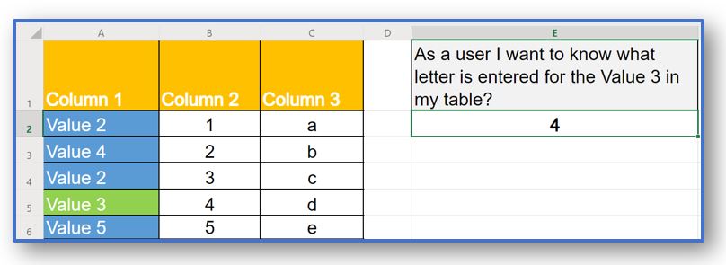
Result is now 4. Why?
When the VLOOKUP Formula uses the binary search it will first check the value in the middle of the table. In Cell A4 Value 2 is (<) smaller than Value 3. Therefore VLOOKUP will check in the next step the lower part of the table again starting in the middle. And voila in cell A5 Value 3 is equal to Value 3. The result is therefore 4.
The VLOOKUP Approximate Match function was developed when the PCs had little computing power. It is the fastest way to search in a table if the values in the table are sorted. This is also the reason why VLOOKUP in the default mode in Excel will use the Approximate Match still today.
=VLOOKUP(“Value 3,A2:C6,) will deliver the same result as =VLOOKUP(“Value 3”,A2:C6,TRUE).
Since our PCs have so much more power the majority of people will use the VLOOKUP Exact Match. But this requires to always set the default mode to FALSE!
An unsorted table
will make VLOOKUP TRUE unstable
Summary:
VLOOKUP Exact Match | VLOOKUP Approximate Match |
Must enter FALSE or 0 to work in this mode | Default Mode: Can leave empty or enter TRUE or 1 |
Will work for most of the use cases | Use to avoid many if functions |
Helps to avoid the #N/A (not found) issue | Use when working with very large data sets – but the data must be sorted |
And that’s it?
Unfortunately this was only the beginning. Usually VLOOKUP is used in more complex data lookup use cases.
Let’s take it step by step….
VLOOKUP across multiple Excel Sheets
This is the most typical use case of the VLOOKUP function.
Let’s start with two sheets first.
Example: The salesperson Sally Seller provides a list of products and number of pieces sold.
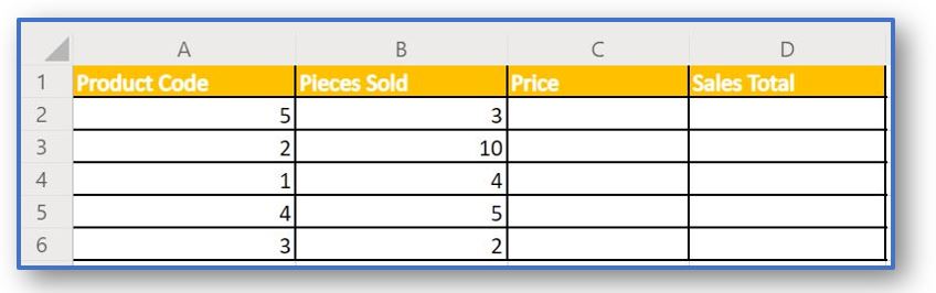
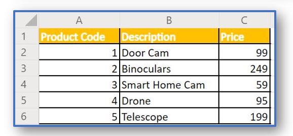
In order to calculate the total sales for Sally Seller the prices are taken from the product price list in the second sheet of the excel file.
To calculate the Total Sales for Sally a Vlookup function is used in Sally’s Sales Table to lookup the product prices in the price list sheet.
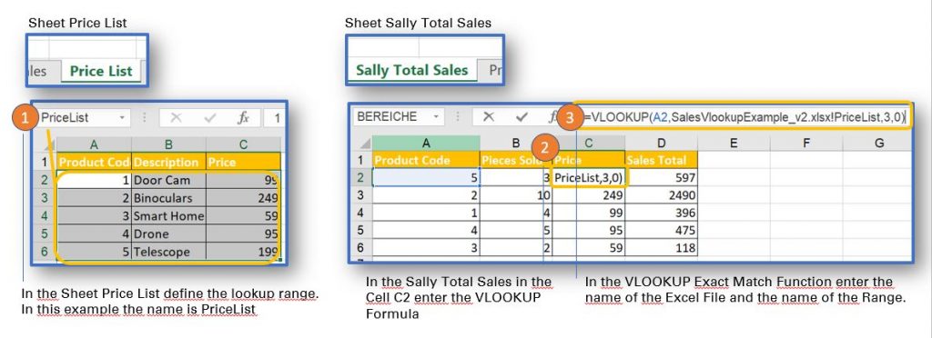
- In the Sheet Price List define a range called PriceList
- In the Sheet Sally Total Sales enter the VLOOKUP function in Cell C2
- The defined range is a unique name within an excel file. To reference the range the name of the excel file needs to be placed before the range name seperated by an exclamation mark ! – In this example the name of the excel file is SalesVlookupExample_v2.xlsx and the name of the range is PriceList.
This Vlookup formula can be used across multiple sheets or across multiple excel files.
If you want to copy & paste the VLOOKUP formula example:
=VLOOKUP(A2,SalesVlookupExample_v2.xlsx!PriceList,3,0)
Instead of a named range an absolute reference can be used. Beware with absolute reference because they are not easy to read and are prone to mistakes.
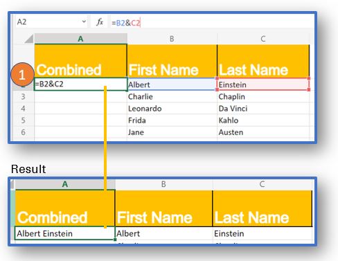
Vlookup function with a helper field
If you want to copy & paste the VLOOKUP formula example:
=VLOOKUP(A2&B2,A2:C6,3,TRUE)
Hello mate, I just wanted to tell you that this article was actually helpful for me. I was fortunate to take the tips you actually so kindly shared and even put it to use. Your web blog article truly aided me and i also would like to inform your dedicated audience that they really have someone that has her or his thoughts fixed. Thank you once more for the excellent posting. I’ve truly bookmarked this on my favored online bookmarking web site and i also recommend everyone else do the very same.